Diffusion of Thought: Chain-of-Thought Reasoning in Diffusion Language Models

논문 정보

• Date: 2025-06-17
• Reviewer: 상엽
• Property: Text Generation, DiffusionLM

https://huggingface.co/blog/ProCreations/diffusion-language-model?utm_source=chatgpt.com

Introduction

도입 배경

• LLM의 엄청난 성장 → Chain-of-Thought (CoT)와 같은 Reasoning이 핵심 기법으로 부상

• CoT는 중간 추론 단계를** autoregressive 방식으로 생성하여 **LLM의 추론 능력을 향상시킴

• 하지만 기존 CoT의 한계점들이 존재

  • 중간 단계의 오류가 최종 답변에 영향을 미침

  • 자기 교정(self-correction) 능력의 부족

  • 효율성에 대한 우려

Diffusion Model의 등장

• Vision 영역에서의 성공에 이어 텍스트 처리 분야에서도 주목받기 시작

• Why? Autoregressive model 대비 고유한 강점을 보유

  • global planning ability

  • self correction

  • 효율성 개선 가능성 (이건 조금 확인이 필요함. 적절한 ref는 아닌 것 같음. https://arxiv.org/pdf/2310.16834)

• Pre-trained diffusion language model → Plaid, SEDD 등 (최근에는 Llama3-8B 정도 수준의 LlaDA 모델 등장)

  • GPT-2 수준의 성능 달성 (DoT는 Neurips 2024 논문)

  • Scaling law의 적용 가능성 확인

RQ

Can diffusion language models also leverage the CoT-style technique to gain enhanced complex reasoning abilities?

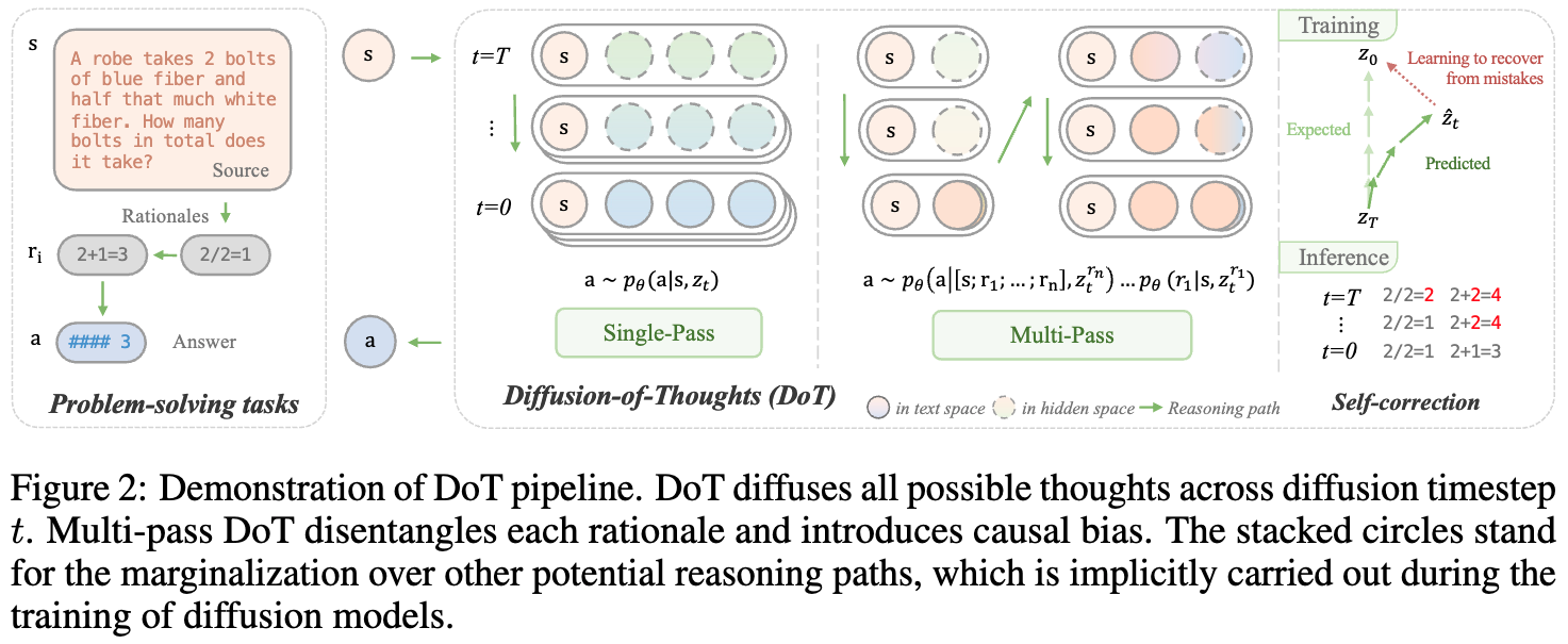
Diffusion of Thoughts (DoT) 제안

• Diffusion model에 특화된 inherent chain-of-thought 방법 제안

  • 일련의 latent variables를 스텝별로 업데이트 → 각 추론 단계들이 시간에 따라 병렬적으로 diffuse

• 핵심 특징

  • Multi-pass variant DoT: causal bias를 막기 위해 한 번에 하나의 thought를 생성하는 데 초점

  • Classifier-free guidance 사용: gradient-based classifier guidance 대신 더 신뢰할 수 있는 제어 신호 제공

  • Training-time sampling: Self-correcting 능력 향상

  • Conditional ODE Solver: continuous diffusion model의 inference 가속

Preliminaries

기본 개념

• Forward process

  • q(\mathbf{z}_t

    \mathbf{z}_{t-1}), t-1 시점의 representation에 noise를 주입

• Reverse process

  • z_{t}를 denoising하여 z_0를 복구하는 것이 목표

  • zt: p{\theta}(\mathbf{z}{0:T}) := p(\mathbf{z}_T)\prod{t=1}^T p{\theta}(\mathbf{z}{t-1}

    \mathbf{z}_t) 로 원본 데이터 복원

• Text generation을 위한 diffusion 모델의 종류

  1. Continuous diffusion models

  • mapping function을 활용 (실수 → 토큰화)

  • discrete text w → continuous space using \text{EMB}(w) → rounding (inverse operation)

  • forward perturbations: q(\mathbf{z}{t} \vert \mathbf{z}{t-1}) = \mathcal{N}(\mathbf{z}{t};\sqrt{1-\beta_t}\mathbf{z}{t-1}, {\beta}_t \mathbf{I}), where \beta_t \in (0, 1)

  1. Discrete diffusion models

  • 문제 자체를 integer program으로 풀기

  • z_t를 ont-hot vectors in {0, 1}^K로 표현. K는 vocab size

  • q(\mathbf{z}_t

    \mathbf{z}_{t-1})을 transition matrix로 표현 → uniform 분포나 [mask]로 전부 변경하는 단계

Seq2Seq Generation (e.g. DiffuSeq)

• 입력-출력 sequence를 single sequence로 처리: \mathbf{w}^{z}=\mathbf{w}^{[x; y]}

• Left-aligned mask [\mathbf{0};\mathbf{1}]로 x, y를 구분

• Partial noising: mask value가 1인 부분에만 noise 적용

Diffusion-of-Thoughts

• Notation: s (problem statement), a (answer), p_{\theta}^{LM} (language model)

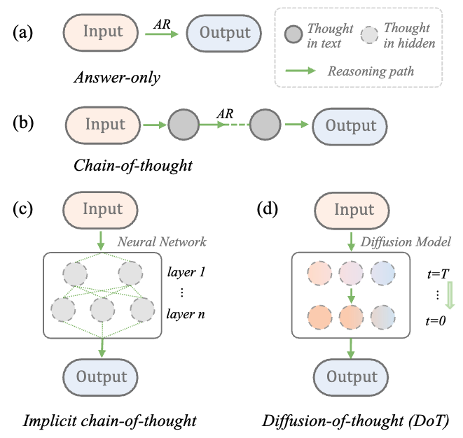
• Answer-only generation model: \mathbf{a}\sim p_\theta^{\textit{LM}}(\mathbf{a}

  \mathbf{s})

• CoT: \mathbf{a}\sim p*\theta^{\textit{LM}}(\mathbf{a}

  \mathbf{s}, \mathbf{r}*{1\dots n})

• implicit CoT: \mathbf{a}\sim p*\theta^{\textit{iCoT}}(\mathbf{a}

  \mathbf{s}, \mathbf{z}*{1\dots n})

• DoT: \mathbf{a}\sim p_\theta^{\textit{DoT}}(\mathbf{a}

  \mathbf{s}, \mathbf{z}_t)

DoT Modeling

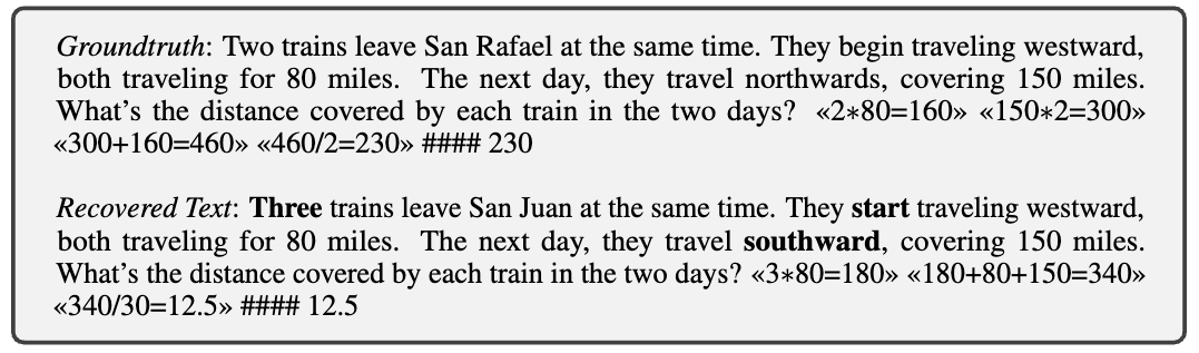
• Gradient-based token guidance의 한계

  • 정확한 conditioning 실패. 특히 수학적 추론과 같이 정확한 숫자와 토큰이 필요한 곳에서 치명적

  • 예시: “Two trains” → “Three trains”

→ DiffuSeq-style classifier-free conditioning 채택

• 모든 rationale들이 backward diffusion process에서 병렬적으로 생성

• 모든 conditional token, 여기서는 s는 고정, r_{1…n}에만 noise 추가

→ continuous 방식의 DiffuSeq-style이 가진 장점이 무엇인가?

• Gradient-based token guidance는 별도의 classifier를 학습 (최근 모델에서는 LLM 내부의 연산을 활용하기도), 여기서 얻은 정보를 condition으로 하여 p의 사후 확률을 조절하는 간접적인 방식

• DiffuSeq 방식은 모델 자체에서 condition (이전 z)를 denoising하는 과정에서 샘플 분포 자체를 확률적으로 조절하는 것으로 더 확실한 변화가 가능

Multi-pass DoT (MP-DoT)

• Causal inductive bias 도입 thought-by-thought 방식으로 rationales을 생성하는 방법 제안

• Process:

  1. \mathbf{r}1\sim p{\theta}^{\textit{DoT}}(\mathbf{r}_1

     \mathbf{s}, \mathbf{z}^{r_1}_t)

  2. \mathbf{r}2\sim p{\theta}^{\textit{DoT}}(\mathbf{r}_2

     [\mathbf{s};\mathbf{r}_1], \mathbf{z}^{r_2}_t)

  3. \mathbf{a}\sim p_{\theta}^{\textit{DoT}}(\mathbf{a}

     [\mathbf{s};\mathbf{r}_1;…;\mathbf{r}_n], \mathbf{z}^{r_n}_t)

• 이후 rationale이 이전 rationale들을 더 강한 condition signal로 이용할 수 있음.

Training

Scheduled Sampling

• Diffusion 모델이 denoising을 하는 과정에서 이미 self-correcting 능력이 있다고 할 수 있음. → Sampling 과정을 통해 이를 더욱 발전

• Training과 inference 간의 exposure bias가 error를 발생시킨다고 생각

• Any timesteps: s, t, u that satisfy 1 < s < t < u < T

  • Training stage: \mathbf{z}_t \sim q(\mathbf{z}_t

    \mathbf{z}_0) (oracle data에서 diffuse)

  • Inference stage: q(z*t

    z*{\theta}(z_u;u))

• 해결책: 추론 단계를 모방하기 위해 \epsilon_i 확률로 다음과 같이 forward step에서 만들어진 z를 활용

  • u \in {t+1, …, T}, \hat{z0} = z{\theta}(z_u;u) → q(z_t

    \hat{z_0})

  • \epsiloni는 1에서 \epsilon{min}로 선형 감소

Coupled Sampling

• Multi-pass DoT에서 rationale에 쌓이는 error accumulation 문제 해결

• Training 시 현재 thought뿐만 아니라 이전 thought들에도 확률적으로 noise 추가

  • \mathbf{z}0=\text{EMB}([\mathbf{s};\mathbf{r}{1};\mathbf{r}_{2}]) 과정에서 일반적으로 r_1에만 noise 적용

  • 일정 확률로 [r_1;r_2] 모두에 noise 적용

Training Objective

DoT 모델에 대해 두 가지 학습 방법을 사용

• from scratch

• fine-tuning from pre-trained diffusion model

공통 Objective function: Negative variational lower bound 최소화

• z_t를 denoising 함으로써 z_0를 복원하는 것을 배우는 것

• Prior loss

  • p_{\theta}(z_T): 최종 noise에서 모델의 분포

  • q(z_T

    w^z): 노이즈를 추가하는 과정에서 만들어진 최종 z의 분포

→ 이상적으론 둘이 동일해져야 하며 prior loss는 0이 되어야 함.

→ 더 직관적으로) 충분히 많은 noise를 주입하면 최종 noise 분포 \mathcal{N(0, I)}가 되어야 함.

• Diffusion loss: 각 단계에서 얼마나 noise를 잘 제거하는가에 대한 탐색

  • 우리가 궁금한 것: p를 통한 denoising이 잘 된 것이 맞을까? == **p{\theta}(z{t-1}

    z_t)** 분포를 잘 구했는가?

  • 우리가 아는 것, z_t (현재 주어진 정보), z_0 (원본)

  • Posterior를 활용, 다음의 분포를 이용해 p_{\theta}를 검정

  • 더 직관적으로 z_{t-1}의 분포가 얼마나 noise, denoise 과정에서 동일한가

• Rounding loss: 복원력 z_0 → \text{w}^z

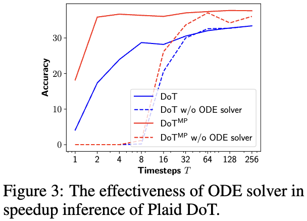
Inference Strategy

• diffusion 모델의 추론 flexibility는 큰 장점 → 어려운 문제일수록 더 많은 reasoning time을 가져야 함. → backward timestep T를 크게 가져가자! (이거 안되는 게 있나? 논문에서 autoregressive 방법에서 토큰 수를 조절하는 것은 더 어렵다고 주장.)

• 문제: Continuous diffusion의 높은 timestep 요구사항 (예: Plaid 4096 timesteps)

→ ODE solver를 conditional form을 활용해 accelerate

• 이게 최종식인데 미분방정식 얘기가 나와서 아직은 모르겠습니다….

Self-consistency Integration

• Multiple sampling을 통한 다양한 reasoning pathway 생성

• 동일 문제 s에 대해 다양한 (r_{i;1…n}, a_i)를 구함. (Diffusion 모델의 강점: noise seed만 다르게 해도 됨!)

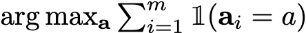
• Majority vote:

Evaluation

Experimental Setup

데이터셋 및 메트릭

• Simple reasoning:

  • 4×4, 5×5 digit multiplication (BIG-bench)

  • Boolean logic reasoning (DyVal)

• Complex reasoning: GSM8K grade school math problems

Base Model

• From scratch: Following DiifuSeq (12-layer Transformer encoder, 124M)

• Pre-trained model for fine-tuning:

  • Plaid (1.3B): OpenWebText에서 훈련, GPT-2 수준 perplexity

  • SEDD-small (170M), SEDD-medium (424M)

Baseline

• Answer-only, CoT, Implicit CoT

• GPT-2 (small 124M, medium 355M, large 774M)

• ChatGPT (gpt-3.5-turbo-1106) with 5-shot CoT

구현 세부사항

• Tokenization: 모든 digit을 개별 토큰으로 처리

• MP-DoT: 마지막 thought 뒤에 <EOS> 토큰 추가 (모델이 rationale 수 결정)

• 8 * V100-32G

• Training:

  • scheduled sampling: \epsilon_{min}=0.95

  • coupled sampling: \gamma (0.01, noise 추가할 확률), k (1, 이전 step)

  • self-consistency: m (20)

• Inference:

  • temperature 0.5, default timestep T: 64

Results

Digit Multiplication & Boolean Logic

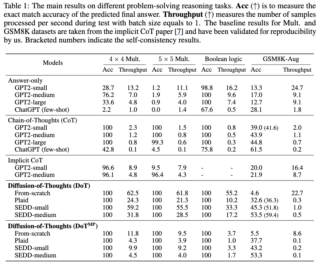
• DoT: 100% 정확도 달성, 이는 CoT를 활용하면 달성할 수 있는 수준

• 속도에서 GPT-2 CoT 대비 최대 27배 빠름.

• **Optimal sampling timestep: 1 for multiplication, 2 for boolean logic **(very EZ)

• ChatGPT와 Implicit CoT도 100% accuracy 달성 실패

→ 간단한 작업에서 DoT의 효율성과 정확성 동시 달성

Results on Complex Reasoning (GSM8K)

• From-scratch training: ~5% accuracy (pre-trained capability의 중요성 확인)

• Fine-tuned DoT: 엄청난 성능 향상

  • SEDD-medium DoT > similar-sized GPT2-medium CoT (10%까지 차이)

  • DoT-SEDD-medium (424M) > GPT2-medium (355M) + CoT

• Multi-pass DoT

  • Plaid에서 single-pass 대비 약간의 성능 향상, 효율성은 single-pass가 우수

  • (성능도 낮고 throughput도 낮아서 이건 왜 한 것인가…)

• Self-consistency: DoT 모델에서 큰 성능 향상

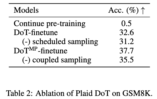
Ablation Study

• Sampling 방법은 효과적

• Continue pre-training (Gradient-based token guidance)를 활용할 경우 0.5%가 됨. (pre-trained 모델보다도 감소)

• Gradient-based conditioning 실패 사례:

• Conditional ODE solver: 4096 → 8 timestep 정도에서 결과 수렴

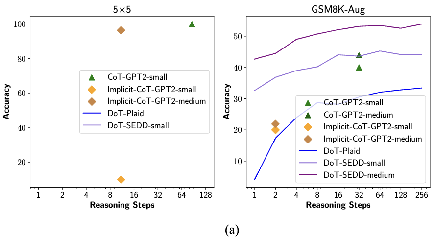
Reasoning-Efficiency Trade-off

• left-to-right 방식의 reasoning을 개선하기 위한 여러 아이디어 (prompting, decoding 등)

• Diffusion도 이러한 reasoning capabilities를 증가시키기 위한 하나의 방안

→ 더 많은 timesteps → 더 많은 reasoning → 효율성 감소

• Efficiency trade-off를 확인

• DoT는 timestep, 나머지 방법은 output token의 수를 step으로 생각

• Simple task (5×5): 1 reasoning step으로 100% accuracy, 추가 computation 불필요

• Complex task (GSM8K): Timestep 증가에 따른 지속적인 성능 향상

  • DoT-SEDD-medium은 outperform

  • DoT-SEDD-small의 경우, 32 timestep에서 GPT2-medium CoT 능가, T=64에서 최고 성능 달성

• **Diffsuion 모델의 장점: **작업 난이도에 따라 timesteps을 자유롭게 조절할 수 있음.

• Autoregressive 한계: CoT와 Implicit CoT는 token-by-token prediction 특성상 명확한 조절이 어려움.

Self-consistency in DoT

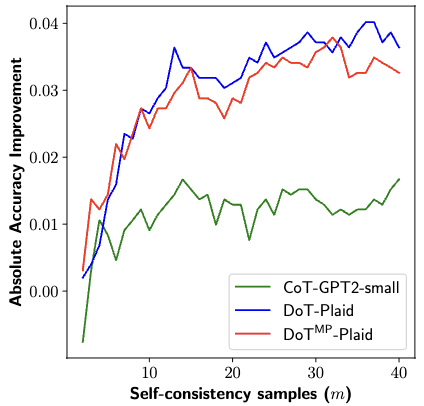
• sampling 수 증가에 따른 지속적 개선

• Autoregressive model과 달리 decoding algorithm 없이도 자연스러운 diversity 제공 (Noise는 다르니깐!)

Self-correction Capability

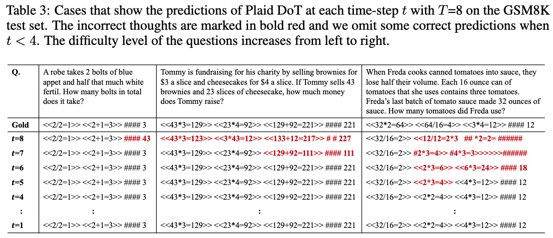
• Autoregressive CoT와 명확히 다른 self-correction 능력을 보임

Case 1: Fast thinking

• 쉬운 문제의 경우, 모든 올바른 thought를 single reasoning step으로 도출

• 두 번째 Step에서 정확한 최종 답변 생성

Case 2: Slow thinking

• 조금 더 어려운 문제 초기에는 에러가 발생

• 후속 단계에서 점진적 refinement를 통한 정확한 답변 도출

• 초기에 문제의 대략적인 outline을 잡고 refine & improve하는 것은 사람의 복잡한 작업 수행 방식과 유사

Case 3: Non-sequential correction

• Step 4: 잘못된 중간 thought <2*3=4> 존재하지만 이후 thought와 답변은 정확

• Step 5: 잘못된 중간 thought 교정

• 핵심 특징: Left-to-right paradigm을 벗어나 좌우의 정보를 바탕으로 수정

Conclusion

• Diffusion model에 특화된 최초의 CoT reasoning 방법 DoT 제안

• Scheduled sampling, coupled sampling, conditional ODE solver 등 고유 기법 개발

• Mathematical reasoning task에서 comprehensive evaluation 수행

---

• Current limitations: Pre-trained diffusion model의 scale과 generalization 한계 (제한된 모델 크기)

• Future promise: 더 강력한 pre-trained model과 함께 autoregressive LLM에 필적하는 성능 기대